Lecture 1: Introduction to Calculus and Limits | PinoyBIX Calculus I Lecture Series

Learning Objectives:

By the end of this lecture, students will be able to:

1. Understand the foundational concept of limits by interpreting function behavior as inputs approach specific values and connecting this to calculus development and real-world applications
2. Evaluate limits using systematic techniques including direct substitution, limit laws, algebraic manipulation (factoring, rationalization), and the Squeeze Theorem for indeterminate forms
3. Analyze function continuity and discontinuities by identifying removable, jump, and infinite discontinuities and determining continuity at specific points and over intervals
4. Apply the Intermediate Value Theorem to prove existence of solutions in engineering problems and understand its role in connecting continuous functions to real-world scenarios
5. Use graphical analysis to support analytical calculations by interpreting limit behavior visually and verifying analytical solutions through multiple approaches
6. Express limit concepts with proper mathematical notation using correct symbols (lim, →, ±∞) and communicate solutions with logical mathematical reasoning and clear explanations

Lecture 1 Outline:

1. Historical Context of Calculus
   • Newton vs. Leibniz controversy
   • Real-world problems that created calculus
2. The Concept of Limits 
   • Intuitive understanding through graphs
   • Formal epsilon-delta definition
   • One-sided limits
3. Limit Laws and Properties
   • Basic limit operations
   • Squeeze theorem application
4. Continuity and Discontinuity
   • Types of discontinuities
   • Intermediate Value Theorem
5. Problem-Solving Practice
   • Worked examples
   • Common limit evaluations

Introduction

Welcome to your first step into the world of calculus – one of the most powerful mathematical tools ever developed. If you’re an engineering student, calculus will become your constant companion throughout your academic journey and professional career. Today, we begin with limits, the foundational concept that makes all of calculus possible.

You might wonder: “Why do I need to learn about limits?” The answer lies in the problems that traditional algebra cannot solve. How do you find the exact slope of a curved line at a single point? How do you calculate the area under a curve that has no simple geometric formula? How do you determine the rate at which a quantity changes when that rate itself is constantly changing?

These questions led to the development of calculus in the 17th century, and they remain relevant today in engineering applications. Whether you’re designing bridges, analyzing electrical circuits, optimizing manufacturing processes, or modeling fluid flow, calculus provides the mathematical framework to solve these complex problems.

In this lecture, we’ll explore limits, the concept that bridges the gap between algebra and calculus. By the end of this session, you’ll understand how limits work, why they matter, and how to evaluate them systematically. More importantly, you’ll see how this seemingly abstract concept connects to real engineering problems you’ll encounter in your career.

Don’t worry if limits seem challenging at first. Every successful engineer has walked this same path. With patience, practice, and the right approach, you’ll master these concepts and build a solid foundation for the calculus journey ahead.

Let’s begin with the fascinating history of how calculus came to be.

1. Historical Context of Calculus

1.1 The Newton-Leibniz Controversy: Two Minds, One Discovery

Calculus emerged in the 17th century through the independent work of two brilliant mathematicians: Isaac Newton and Gottfried Wilhelm Leibniz. This development represents one of mathematics’ most significant achievements and sparked one of history’s most famous intellectual disputes.

Isaac Newton’s Approach (1665-1667)

Newton developed his “method of fluxions” while studying at Cambridge University. His approach focused on:

• Motion and changing quantities (which he called “fluents”)
• Rates of change (which he termed “fluxions”)
• Physical applications, particularly planetary motion and optics

Newton’s notation used dots above variables to represent derivatives (ẋ for dx/dt), which reflected his physics-oriented thinking.

Gottfried Leibniz’s Contribution (1674-1676)

Leibniz developed calculus through a more systematic mathematical framework:

• Created the dx and dy notation we use today
• Developed the integral sign (∫) based on the letter “S” for “sum”
• Emphasized the mathematical rigor and symbolic manipulation

The controversy arose because Newton developed his methods earlier but published later, while Leibniz published first but developed his methods later. This led to accusations of plagiarism and a bitter dispute between English and Continental European mathematicians.

1.2 Real-world problems that drove calculus development:

Planetary Motion and Astronomy

The need to understand orbital mechanics drove much of calculus development. Kepler’s laws described planetary motion, but explaining why planets followed these paths required calculus. Newton used his calculus to derive the inverse square law of gravitation and explain planetary orbits.

Optics and Light Behavior

Problems in optics, such as finding the path light takes when traveling through different media, required optimization techniques that became fundamental calculus applications. Fermat’s principle of least time needed calculus for its mathematical proof.

Area and Volume Calculations

Ancient problems of finding areas under curves and volumes of irregular shapes found elegant solutions through integral calculus. The method of exhaustion used by ancient Greeks was essentially early integral calculus.

Optimization Problems

Finding maximum cannon range or minimum material usage in construction presented practical challenges that demanded systematic mathematical approaches. Military engineers needed to determine the optimal angle for cannon trajectories to achieve maximum range, while architects and builders sought to minimize material costs while maintaining structural integrity. These optimization problems required techniques for finding maximum and minimum values of functions, fundamental applications of differential calculus.

Rate Problems

Understanding how quantities change over time in physics and engineering became increasingly important as technology advanced. Questions like “How fast does water flow out of a tank?” or “At what rate does a falling object accelerate?” require mathematical tools to describe instantaneous rates of change. These problems led to the development of derivatives as measures of how one quantity changes with respect to another.

Engineering and Construction

Building bridges, fortifications, and ships required an understanding of the strength of materials, fluid flow, and structural optimization – all problems that calculus would eventually solve systematically.

2. The Concept of Limits

2.1 Intuitive Understanding Through Graphical Analysis

The limit concept answers the question: “What value does a function approach as the input gets arbitrarily close to a specific point?”

Visual Understanding

Consider the function f(x) = (x² – 1)/(x – 1). When x = 1, we get 0/0, which is undefined. However, we can examine what happens as x approaches 1:

• When x = 1.1: f(x) = 2.1
• When x = 1.01: f(x) = 2.01
• When x = 1.001: f(x) = 2.001

From the left side:

• When x = 0.9: f(x) = 1.9
• When x = 0.99: f(x) = 1.99
• When x = 0.999: f(x) = 1.999

The function approaches 2 as x approaches 1, even though f(1) is undefined.

Graphical Interpretation

On a graph, limits represent the y-value that the function approaches as you trace along the curve toward a specific x-value. The actual function value at that point may be different from the limit, or may not exist at all.

2.2 Formal Epsilon-Delta Definition

The rigorous mathematical definition of limits uses the epsilon-delta (ε-δ) framework:

Definition: The limit of f(x) as x approaches a equals L if:

For every ε > 0, there exists a δ > 0 such that whenever 0 < |x – a| < δ, then |f(x) – L| < ε.

Breaking Down the Definition:

• ε (epsilon) represents how close we want f(x) to be to L
• δ (delta) represents how close x must be to a
• The definition says: “No matter how small you make ε, I can find a δ that works.”

Practical Understanding:

Think of this as a challenge-response game:

1. Someone challenges you with an ε (how accurate they want the answer)
2. You respond with a δ (how close x needs to be to a)
3. You win if staying within δ of a guarantees staying within ε of L

2.3 One-Sided Limits and Their Significance

Left-Hand Limits

Written as lim(x→a⁻) f(x), this represents the limit as x approaches a from values less than a.

Right-Hand Limits

Written as lim(x→a⁺) f(x), this represents the limit as x approaches a from values greater than a.

Relationship to Two-Sided Limits

A two-sided limit exists if and only if both one-sided limits exist and are equal:

lim(x→a) f(x) = L if and only if lim(x→a⁻) f(x) = lim(x→a⁺) f(x) = L

Engineering Significance

One-sided limits are crucial in engineering because:

• Physical systems often behave differently when approaching from different directions
• Control systems may have different responses for increasing vs. decreasing inputs
• Material properties can exhibit different behaviors under loading vs. unloading

Example: For f(x) = |x|/x:

From the left (x < 0): f(x) = -1, so lim(x→0⁻) f(x) = -1

From the right (x > 0): f(x) = 1, so lim(x→0⁺) f(x) = 1

Since -1 ≠ 1, lim(x→0) f(x) does not exist

3. Limit Laws and Properties

Once you understand basic limits, these laws make evaluation much easier:

3.1 Fundamental Limit Laws:

1. Constant Law: lim(x→a) c = c

2. Identity Law: lim(x→a) x = a

3. Sum Law: lim(x→a) [f(x) + g(x)] = lim(x→a) f(x) + lim(x→a) g(x)

• The limit of a sum equals the sum of the limits (when both limits exist).

4. Difference Law: lim(x→a) [f(x) – g(x)] = lim(x→a) f(x) – lim(x→a) g(x)

5. Product Law: lim(x→a) [f(x) · g(x)] = [lim(x→a) f(x)] · [lim(x→a) g(x)]

6. Quotient Law: lim(x→a) [f(x)/g(x)] = [lim(x→a) f(x)] / [lim(x→a) g(x)], provided lim(x→a) g(x) ≠ 0

7. Constant Multiple Rule: lim(x→a) [c · f(x)] = c · lim(x→a) f(x), where c is any constant

8. Power Rule: lim(x→a) [f(x)]ⁿ = [lim(x→a) f(x)]ⁿ, where n is a positive integer

Example Application: Find lim(x→3) (2x² + 5x – 1)

Using limit laws:

= lim(x→3) 2x² + lim(x→3) 5x – lim(x→3) 1

= 2[lim(x→3) x]² + 5[lim(x→3) x] – 1

= 2(3)² + 5(3) – 1

= 18 + 15 – 1 = 32

3.2 The Squeeze Theorem:

This powerful tool helps evaluate limits that seem impossible to find directly.

Statement of the Theorem

If g(x) ≤ f(x) ≤ h(x) for all x in some interval containing a (except possibly at a), and if lim(x→a) g(x) = lim(x→a) h(x) = L, then lim(x→a) f(x) = L.

Intuitive Understanding

Imagine f(x) as being “squeezed” between two other functions g(x) and h(x). If the two bounding functions approach the same limit, then the squeezed function must also approach that same limit.

Applications of the Squeeze Theorem

Classic Example 1: lim(x→0) (sin x)/x = 1

This fundamental limit is proved using the squeeze theorem:

For 0 < x < π/2: cos x < (sin x)/x < 1

As x → 0: cos x → 1 and 1 → 1

Therefore: (sin x)/x → 1

Classic Example 2: Find lim(x→0) x sin(1/x)

We know that -1 ≤ sin(1/x) ≤ 1 for all x ≠ 0.

Multiplying by |x|: -|x| ≤ x sin(1/x) ≤ |x|

Since lim(x→0) (-|x|) = 0 and lim(x→0) |x| = 0, by the squeeze theorem:

lim(x→0) x sin(1/x) = 0

Therefore: x sin(1/x) → 0

Engineering Applications

• Vibration analysis where oscillating functions are bounded
• Error analysis in numerical methods
• Signal processing applications with bounded noise

4. Continuity and Discontinuity

Definition of Continuity

A function f(x) is continuous at x = a if three conditions are met:

1. f(a) exists (the function is defined at a)
2. lim(x→a) f(x) exists (the limit exists)
3. lim(x→a) f(x) = f(a) (the limit equals the function value)

Practical Interpretation

A function is continuous if you can draw its graph without lifting your pencil from the paper.

4.1 Types of Discontinuities:

Removable Discontinuity (Point Discontinuity)

• The limit exists, but either f(a) doesn’t exist or f(a) ≠ lim(x→a) f(x)
• The limit exists but doesn’t equal the function value.
• Can be “fixed” by redefining the function at that point
• Example: f(x) = (x² – 1)/(x – 1) at x = 1 The limit is 2, but f(1) is undefined.

Jump Discontinuity

• Left and right limits exist but are not equal
• Common in piecewise functions
• Example: The unit step function in engineering at x = 0

Infinite Discontinuity

• At least one of the one-sided limits is infinite
• Occurs at vertical asymptotes
• Example: f(x) = 1/(x – 2) at x = 2

Oscillating Discontinuity

• The limit does not exist because the function oscillates
• Example: f(x) = sin(1/x) at x = 0

4.2 Intermediate Value Theorem:

This theorem guarantees that continuous functions take on all intermediate values.

Theorem Statement

If f is continuous on the closed interval [a, b] and N is any number between f(a) and f(b), then there exists at least one number c in (a, b) such that f(c) = N.

Practical Significance

This theorem guarantees that continuous functions take on all intermediate values.  In engineering terms, if a system starts in one state and ends in another, it must pass through all intermediate states if the transition is continuous.

This theorem proves that equations have solutions.

For example, to show that x³ – x – 1 = 0 has a solution, note that f(x) = x³ – x – 1 is continuous, f(1) = -1 < 0, and f(2) = 5 > 0. By IVT, there’s a root between 1 and 2.

Applications

• Root-finding algorithms (bisection method)
• Existence proofs for solutions to equations
• Design verification in control systems

5. Problem-Solving Techniques

5.1 Algebraic Methods for Evaluating Limits

Direct Substitution

Try substituting the limit value directly into the function. If this gives a definite answer (not 0/0 or ∞/∞), then that’s your limit.

Factoring and Canceling

When direct substitution gives 0/0:

• Factor both the numerator and the denominator
• Cancel common factors
• Substitute the limit value

Example: lim(x→2) (x² – 4)/(x – 2) = lim(x→2) (x + 2)(x – 2)/(x – 2) = lim(x→2) (x + 2) = 4

Rationalizing

For limits involving square roots that give 0/0:

• Multiply by the conjugate
• Simplify the resulting expression
• Substitute the limit value

Example: lim(x→0) (√(x + 1) – 1)/x

Multiply by (√(x + 1) + 1)/(√(x + 1) + 1):

= lim(x→0) (x + 1 – 1)/[x(√(x + 1) + 1)]

= lim(x→0) x/[x(√(x + 1) + 1)]

= lim(x→0) 1/(√(x + 1) + 1) = 1/2

5.2 Graphical Analysis Techniques

Using Function Behavior

• Identify the domain and range of the function
• Look for asymptotes (vertical, horizontal, oblique)
• Examine the function’s behavior near critical points
• Use symmetry properties when applicable

Piecewise Function Analysis

For piecewise functions:

• Identify which piece applies near the limit point
• Check continuity at boundary points
• Evaluate one-sided limits separately if needed

5.3 Common Limit Patterns

Polynomial Functions

• Always continuous everywhere
• Limits can be found by direct substitution
• lim(x→a) P(x) = P(a) for any polynomial P

Rational Functions

• Continuous except where the denominator equals zero
• At points where the denominator is zero, check if the numerator is also zero
• If both approach zero, factor and simplify

Trigonometric Functions

• sin x and cos x are continuous everywhere
• tan x has discontinuities where cos x = 0
• Key limit: lim(x→0) (sin x)/x = 1

5.4 Engineering Applications

5.4.1 Circuit Analysis

RC Circuit Charging

In an RC circuit, the voltage across the capacitor follows:

V_C(t) = V_0(1 – e^(-t/RC))

• The limit as t → ∞ gives the steady-state voltage:
• lim(t→∞) V_C(t) = V_0
• This limit helps engineers determine the final state of charging circuits.

Transfer Function Analysis

In control systems, transfer functions H(s) have limits that determine system behavior:

• lim(s→0) H(s) gives DC gain
• lim(s→∞) H(s) determines high-frequency response

5.4.2 Structural Engineering

Beam Deflection

The deflection of a loaded beam can be expressed as a function that may have discontinuities at load points. Limits help determine:

• Maximum deflection points
• Continuity of the deflection curve
• Slope changes at load discontinuities

Material Properties

Stress-strain relationships often involve limits:

• Elastic limit (yield strength)
• Ultimate strength limits
• Fatigue limits under cyclic loading

5.4.3 Signal Processing

Sampling Theory

The sinc function sin(πt)/(πt) has the important limit:

lim(t→0) sin(πt)/(πt) = 1

This limit is fundamental to understanding signal reconstruction and the sampling theorem.

Filter Design

Frequency response functions H(ω) use limits to determine:

• Passband and stopband behavior
• Cutoff frequency characteristics
• Phase response at critical frequencies

5.4.4 Fluid Mechanics

Boundary Layer Theory

Velocity profiles in boundary layers involve limits:

• Velocity approaches zero at solid boundaries
• Velocity approaches the free-stream value away from the boundaries
• Shear stress calculations depend on velocity gradients (limits)

Pipe Flow Analysis

Pressure drop calculations in pipe flow systems use limits to:

• Determine the entrance length effects
• Calculate fully developed flow characteristics
• Analyze the transition between laminar and turbulent flow

Basic Limit Evaluation

Example 1: Evaluate lim(x→2) (x² – 4)/(x – 2)

Technique Used: Factoring to resolve indeterminate form 0/0

Step-by-Step Solution:

1. Check direct substitution: (2)² – 4)/(2 – 2) = 0/0 (indeterminate form)
2. Factor the numerator using difference of squares: x² – 4 = (x + 2)(x – 2)
3. Rewrite the expression: (x + 2)(x – 2)/(x – 2)
4. Cancel common factors: (x + 2)(x – 2)/(x – 2) = x + 2 (for x ≠ 2)
5. Evaluate the limit: lim(x→2) (x + 2) = 2 + 2 = 4

Answer: The limit is 4.

Example 2: Evaluate lim(x→∞) (3x² + 2x + 1)/(x² – x + 5)

Technique Used: Dividing by the highest power for limits at infinity

Step-by-Step Solution:

1. Identify the highest power in the denominator: x²
2. Divide both the numerator and denominator by x²:
   • Numerator: (3x² + 2x + 1)/x² = 3 + 2/x + 1/x²
   • Denominator: (x² – x + 5)/x² = 1 – 1/x + 5/x²
3. Rewrite the limit: lim(x→∞) (3 + 2/x + 1/x²)/(1 – 1/x + 5/x²)
4. Apply limit properties as x → ∞: 2/x → 0, 1/x² → 0, 1/x → 0, 5/x² → 0
5. Evaluate: (3 + 0 + 0)/(1 – 0 + 0) = 3/1 = 3

Answer: The limit is 3.

Example 3: Find where f(x) = (x² – 1)/(x – 1) is discontinuous and classify the discontinuity

Technique Used: Analyzing discontinuities by finding undefined points and limits

Step-by-Step Solution:

1. Find where function is undefined: x – 1 = 0, so x = 1
2. Factor the numerator: x² – 1 = (x + 1)(x – 1)
3. Simplify the function: f(x) = (x + 1)(x – 1)/(x – 1) = x + 1 (for x ≠ 1)
4. Find the limit as x approaches 1: lim(x→1) (x + 1) = 1 + 1 = 2
5. Classify discontinuity: Since the limit exists but f(1) is undefined, this is a removable discontinuity

Answer: Removable discontinuity at x = 1.

Example 4: Evaluate lim(x→3) (x² + 2x – 15)/(x – 3)

Technique Used: Factoring a quadratic to resolve the 0/0 indeterminate form

Step-by-Step Solution:

1. Check direct substitution: (9 + 6 – 15)/(3 – 3) = 0/0 (indeterminate)
2. Factor the numerator x² + 2x – 15: Find two numbers that multiply to -15 and add to 2
3. The numbers are 5 and -3: x² + 2x – 15 = (x + 5)(x – 3)
4. Rewrite the expression: (x + 5)(x – 3)/(x – 3)
5. Cancel common factors: (x + 5) for x ≠ 3
6. Evaluate the limit: lim(x→3) (x + 5) = 3 + 5 = 8

Answer: The limit is 8.

Example 5: Find lim(x→0) sin(x)/x using the squeeze theorem

Technique Used: Squeeze theorem with geometric analysis

Step-by-Step Solution:

1. Recognize this as a fundamental trigonometric limit
2. Use geometric approach: For 0 < x < π/2, construct a unit circle sector
3. Compare areas: Area of triangle < Area of sector < Area of larger triangle
4. This gives us: sin(x) < x < tan(x) for small positive x
5. Divide by sin(x): 1 < x/sin(x) < 1/cos(x)
6. Take reciprocals (flip inequalities): cos(x) < sin(x)/x < 1
7. Apply squeeze theorem: lim(x→0) cos(x) = 1 and lim(x→0) 1 = 1
8. Therefore: lim(x→0) sin(x)/x = 1

Answer: The limit is 1.

Radical and Conjugate Problems

Example 6: Evaluate lim(x→4) (√x – 2)/(x – 4)

Technique Used: Rationalization using conjugate multiplication

Step-by-Step Solution:

1. Check direct substitution: (√4 – 2)/(4 – 4) = 0/0 (indeterminate)
2. Multiply by conjugate: (√x – 2)/(x – 4) × (√x + 2)/(√x + 2)
3. Apply difference of squares in numerator: (√x)² – 2² = x – 4
4. Simplify: (x – 4)/[(x – 4)(√x + 2)]
5. Cancel common factors: 1/(√x + 2) for x ≠ 4
6. Evaluate the limit: lim(x→4) 1/(√x + 2) = 1/(√4 + 2) = 1/(2 + 2) = 1/4

Answer: The limit is 1/4.

Example 7: Find lim(x→∞) (2x³ – x² + 1)/(5x³ + 3x – 7)

Technique Used: Dividing by the highest power for rational functions

Step-by-Step Solution:

1. Identify the highest powers: Both the numerator and denominator have degree 3
2. Divide both by x³:
   • Numerator: (2x³ – x² + 1)/x³ = 2 – 1/x + 1/x³
   • Denominator: (5x³ + 3x – 7)/x³ = 5 + 3/x² – 7/x³
3. Rewrite limit: lim(x→∞) (2 – 1/x + 1/x³)/(5 + 3/x² – 7/x³)
4. Apply limit properties: All terms with x in the denominator approach 0
5. Evaluate: (2 – 0 + 0)/(5 + 0 – 0) = 2/5

Answer: The limit is 2/5.

Example 8: Evaluate lim(x→-2) (x³ + 8)/(x + 2)

Technique Used: Sum of cubes factoring

Step-by-Step Solution:

1. Check direct substitution: ((-2)³ + 8)/(-2 + 2) = 0/0 (indeterminate)
2. Recognize x³ + 8 as sum of cubes: x³ + 2³
3. Apply sum of cubes formula: a³ + b³ = (a + b)(a² – ab + b²)
4. Factor: x³ + 8 = (x + 2)(x² – 2x + 4)
5. Simplify: (x + 2)(x² – 2x + 4)/(x + 2) = x² – 2x + 4 for x ≠ -2
6. Evaluate: lim(x→-2) (x² – 2x + 4) = (-2)² – 2(-2) + 4 = 4 + 4 + 4 = 12

Answer: The limit is 12.

Example 9: Find lim(x→1) (x^n – 1)/(x – 1) where n is a positive integer

Technique Used: General factorization of x^n – 1

Step-by-Step Solution:

1. Check direct substitution: (1^n – 1)/(1 – 1) = 0/0 (indeterminate)
2. Use factorization: x^n – 1 = (x – 1)(x^(n-1) + x^(n-2) + … + x + 1)
3. Rewrite the expression: (x – 1)(x^(n-1) + x^(n-2) + … + x + 1)/(x – 1)
4. Cancel common factors: x^(n-1) + x^(n-2) + … + x + 1 for x ≠ 1
5. Count terms in the sum: There are n terms (from x^(n-1) down to x^0)
6. Evaluate: lim(x→1) (x^(n-1) + x^(n-2) + … + x + 1) = 1 + 1 + … + 1 = n

Answer: The limit is n.

Trigonometric Limits

Example 10: Evaluate lim(x→0) (1 – cos(x))/x²

Technique Used: Half-angle identity and fundamental limits

Step-by-Step Solution:

1. Check direct substitution: (1 – cos(0))/0² = 0/0 (indeterminate)
2. Use half-angle identity: 1 – cos(x) = 2sin²(x/2)
3. Substitute: lim(x→0) 2sin²(x/2)/x²
4. Rewrite x² as 4(x/2)²: lim(x→0) 2sin²(x/2)/[4(x/2)²]
5. Factor out constants: lim(x→0) (1/2)[sin(x/2)/(x/2)]²
6. Apply fundamental limit lim(u→0) sin(u)/u = 1 where u = x/2:
7. Evaluate: (1/2) × 1² = 1/2

Answer: The limit is 1/2.

Example 11: Find lim(x→0⁺) x ln(x)

Technique Used: Rewriting indeterminate form and L’Hôpital’s rule preview

Step-by-Step Solution:

1. Identify indeterminate form: 0 × (-∞)
2. Rewrite as quotient: lim(x→0⁺) ln(x)/(1/x) which gives -∞/∞
3. Apply L’Hôpital’s rule: Differentiate numerator and denominator
   • d/dx[ln(x)] = 1/x
   • d/dx[1/x] = -1/x²
4. New limit: lim(x→0⁺) (1/x)/(-1/x²) = lim(x→0⁺) (1/x) × (-x²) = lim(x→0⁺) (-x)
5. Evaluate: lim(x→0⁺) (-x) = 0

Answer: The limit is 0.

Example 12: Evaluate lim(x→∞) (√(x² + 1) – x)

Technique Used: Conjugate multiplication for ∞ – ∞ form

Step-by-Step Solution:

1. Identify indeterminate form: ∞ – ∞
2. Multiply by conjugate: (√(x² + 1) – x) × (√(x² + 1) + x)/(√(x² + 1) + x)
3. Apply difference of squares: [(√(x² + 1))² – x²]/[√(x² + 1) + x]
4. Simplify numerator: (x² + 1 – x²)/[√(x² + 1) + x] = 1/[√(x² + 1) + x]
5. As x → ∞: both √(x² + 1) → ∞ and x → ∞
6. Evaluate: lim(x→∞) 1/[√(x² + 1) + x] = 1/∞ = 0

Answer: The limit is 0.

Example 13: Find lim(x→2) (x – 2)/(x² – 4)

Technique Used: Factoring denominator

Step-by-Step Solution:

1. Check direct substitution: (2 – 2)/(2² – 4) = 0/0 (indeterminate)
2. Factor the denominator: x² – 4 = (x – 2)(x + 2)
3. Rewrite: (x – 2)/[(x – 2)(x + 2)]
4. Cancel common factors: 1/(x + 2) for x ≠ 2
5. Evaluate: lim(x→2) 1/(x + 2) = 1/(2 + 2) = 1/4

Answer: The limit is 1/4.

Example 14: Evaluate lim(x→0) tan(x)/x

Technique Used: Rewriting tangent and using fundamental limits

Step-by-Step Solution:

1. Rewrite tangent: tan(x) = sin(x)/cos(x)
2. Substitute: lim(x→0) tan(x)/x = lim(x→0) sin(x)/(x cos(x))
3. Separate the fraction: lim(x→0) [sin(x)/x] × [1/cos(x)]
4. Apply limit properties: lim(x→0) sin(x)/x × lim(x→0) 1/cos(x)
5. Use fundamental limits: lim(x→0) sin(x)/x = 1 and lim(x→0) 1/cos(x) = 1/cos(0) = 1
6. Evaluate: 1 × 1 = 1

Answer: The limit is 1.

Example 15: Find lim(x→∞) x/(√(x² + 1))

Technique Used: Dividing by the highest power under radical

Step-by-Step Solution:

1. Factor out x from the radical: √(x² + 1) = √(x²(1 + 1/x²)) = |x|√(1 + 1/x²)
2. For x > 0 as x → ∞: |x| = x, so √(x² + 1) = x√(1 + 1/x²)
3. Substitute: lim(x→∞) x/[x√(1 + 1/x²)]
4. Cancel x: lim(x→∞) 1/√(1 + 1/x²)
5. Apply limit: lim(x→∞) 1/x² = 0
6. Evaluate: 1/√(1 + 0) = 1/√1 = 1

Answer: The limit is 1.

Exponential and Logarithmic Limits

Example 16: Evaluate lim(x→0) (e^x – 1)/x

Technique Used: Fundamental exponential limit

Step-by-Step Solution:

1. Check direct substitution: (e^0 – 1)/0 = 0/0 (indeterminate)
2. Recognize as fundamental limit: This is the definition of the derivative of e^x at x = 0
3. Recall that d/dx[e^x] = e^x, so d/dx[e^x]|_{x=0} = e^0 = 1
4. By definition of derivative: lim(h→0) (e^h – e^0)/h = lim(h→0) (e^h – 1)/h
5. Therefore: lim(x→0) (e^x – 1)/x = 1

Answer: The limit is 1.

Example 17: Find lim(x→0) sin(3x)/sin(5x)

Technique Used: Rewriting using fundamental trigonometric limits

Step-by-Step Solution:

1. Check direct substitution: sin(0)/sin(0) = 0/0 (indeterminate)
2. Rewrite by multiplying and dividing strategically:
   • lim(x→0) sin(3x)/sin(5x) × (3x/3x) × (5x/5x)
3. Rearrange: lim(x→0) [sin(3x)/3x] × [5x/sin(5x)] × [3x/5x]
4. Apply fundamental limit lim(u→0) sin(u)/u = 1:
   • lim(x→0) sin(3x)/3x = 1 (where u = 3x)
   • lim(x→0) 5x/sin(5x) = 1 (reciprocal of fundamental limit where u = 5x)
5. Evaluate: 1 × 1 × (3/5) = 3/5

Answer: The limit is 3/5.

Example 18: Evaluate lim(x→∞) (3x + 1)/(2x – 5)

Technique Used: Dividing by the highest power

Step-by-Step Solution:

1. Identify the highest power: x (degree 1 in both numerator and denominator)
2. Divide both by x:
   • Numerator: (3x + 1)/x = 3 + 1/x
   • Denominator: (2x – 5)/x = 2 – 5/x
3. Rewrite: lim(x→∞) (3 + 1/x)/(2 – 5/x)
4. Apply limits: lim(x→∞) 1/x = 0 and lim(x→∞) 5/x = 0
5. Evaluate: (3 + 0)/(2 – 0) = 3/2

Answer: The limit is 3/2.

Example 19: Find lim(x→4) (2 – √x)/(4 – x)

Technique Used: Conjugate multiplication and algebraic manipulation

Step-by-Step Solution:

1. Check direct substitution: (2 – √4)/(4 – 4) = 0/0 (indeterminate)
2. Note that 4 – x = -(x – 4) for easier manipulation
3. Multiply by conjugate: (2 – √x)/(-(x – 4)) × (2 + √x)/(2 + √x)
4. Apply difference of squares: (4 – x)/[-(x – 4)(2 + √x)]
5. Substitute 4 – x = -(x – 4): [-(x – 4)]/[-(x – 4)(2 + √x)]
6. Cancel: -1/(2 + √x) for x ≠ 4
7. Evaluate: lim(x→4) [-1/(2 + √x)] = -1/(2 + √4) = -1/(2 + 2) = -1/4

Answer: The limit is -1/4.

Example 20: Evaluate lim(x→0) (√(1 + x) – 1)/x

Technique Used: Conjugate multiplication

Step-by-Step Solution:

1. Check direct substitution: (√1 – 1)/0 = 0/0 (indeterminate)
2. Multiply by conjugate: (√(1 + x) – 1)/x × (√(1 + x) + 1)/(√(1 + x) + 1)
3. Apply difference of squares in numerator: [(1 + x) – 1]/[x(√(1 + x) + 1)]
4. Simplify numerator: x/[x(√(1 + x) + 1)]
5. Cancel x: 1/(√(1 + x) + 1) for x ≠ 0
6. Evaluate: lim(x→0) 1/(√(1 + x) + 1) = 1/(√1 + 1) = 1/(1 + 1) = 1/2

Answer: The limit is 1/2.

Advanced Factoring and Algebraic Manipulation

Example 21: Evaluate lim(x→5) (x³ – 125)/(x – 5)

Technique Used: Difference of cubes factoring

Step-by-Step Solution:

1. Check direct substitution: (125 – 125)/(5 – 5) = 0/0 (indeterminate)
2. Recognize x³ – 125 as difference of cubes: x³ – 5³
3. Apply difference of cubes formula: a³ – b³ = (a – b)(a² + ab + b²)
4. Factor: x³ – 125 = (x – 5)(x² + 5x + 25)
5. Substitute: (x – 5)(x² + 5x + 25)/(x – 5)
6. Cancel: x² + 5x + 25 for x ≠ 5
7. Evaluate: lim(x→5) (x² + 5x + 25) = 25 + 25 + 25 = 75

Answer: The limit is 75.

Example 22: Find lim(x→-1) (x⁴ – 1)/(x + 1)

Technique Used: Multiple factorization steps

Step-by-Step Solution:

1. Check direct substitution: (1 – 1)/(-1 + 1) = 0/0 (indeterminate)
2. Factor x⁴ – 1 as difference of squares: (x²)² – 1² = (x² – 1)(x² + 1)
3. Factor x² – 1 further: (x – 1)(x + 1)
4. Complete factorization: x⁴ – 1 = (x – 1)(x + 1)(x² + 1)
5. Substitute: (x – 1)(x + 1)(x² + 1)/(x + 1)
6. Cancel: (x – 1)(x² + 1) for x ≠ -1
7. Evaluate: lim(x→-1) (x – 1)(x² + 1) = (-1 – 1)(1 + 1) = (-2)(2) = -4

Answer: The limit is -4.

Example 23: Evaluate lim(x→0) (x² + 3x)/x

Technique Used: Factoring common terms

Step-by-Step Solution:

1. Check direct substitution: (0 + 0)/0 = 0/0 (indeterminate)
2. Factor numerator: x² + 3x = x(x + 3)
3. Substitute: x(x + 3)/x
4. Cancel x: x + 3 for x ≠ 0
5. Evaluate: lim(x→0) (x + 3) = 0 + 3 = 3

Answer: The limit is 3.

Example 24: Find lim(x→2) (x³ – 8)/(x² – 4)

Technique Used: Factoring both numerator and denominator

Step-by-Step Solution:

1. Check direct substitution: (8 – 8)/(4 – 4) = 0/0 (indeterminate)
2. Factor numerator (difference of cubes): x³ – 8 = x³ – 2³ = (x – 2)(x² + 2x + 4)
3. Factor denominator (difference of squares): x² – 4 = (x – 2)(x + 2)
4. Substitute: (x – 2)(x² + 2x + 4)/[(x – 2)(x + 2)]
5. Cancel common factor: (x² + 2x + 4)/(x + 2) for x ≠ 2
6. Evaluate: lim(x→2) (x² + 2x + 4)/(x + 2) = (4 + 4 + 4)/(2 + 2) = 12/4 = 3

Answer: The limit is 3.

Example 25: Evaluate lim(x→3) (x² – 9)/(√(x + 1) – 2)

Technique Used: Factoring numerator and rationalizing denominator

Step-by-Step Solution:

1. Check direct substitution: (9 – 9)/(√4 – 2) = 0/0 (indeterminate)
2. Factor numerator: x² – 9 = (x – 3)(x + 3)
3. Rationalize denominator by multiplying by conjugate:
   • (√(x + 1) – 2) × (√(x + 1) + 2)/(√(x + 1) + 2)
4. Denominator becomes: (x + 1) – 4 = x – 3
5. Original expression becomes: (x – 3)(x + 3)/[(x – 3)/(√(x + 1) + 2)]
6. Simplify: (x – 3)(x + 3) × (√(x + 1) + 2)/(x – 3) = (x + 3)(√(x + 1) + 2)
7. Evaluate: lim(x→3) (x + 3)(√(x + 1) + 2) = (3 + 3)(√4 + 2) = 6 × 4 = 24

Answer: The limit is 24.

Limits Involving Absolute Values

Example 26: Find lim(x→0) |x|/x

Technique Used: One-sided limits analysis

Step-by-Step Solution:

1. Recognize that |x|/x behaves differently on each side of x = 0
2. Calculate left-hand limit: lim(x→0⁻) |x|/x
   • For x < 0: |x| = -x
   • So lim(x→0⁻) |x|/x = lim(x→0⁻) (-x)/x = lim(x→0⁻) (-1) = -1
3. Calculate right-hand limit: lim(x→0⁺) |x|/x
   • For x > 0: |x| = x
   • So lim(x→0⁺) |x|/x = lim(x→0⁺) x/x = lim(x→0⁺) 1 = 1
4. Compare one-sided limits: -1 ≠ 1
5. Conclusion: Since left and right limits differ, the limit does not exist

Answer: The limit does not exist.

Example 27: Evaluate lim(x→2) |x – 2|/(x² – 4)

Technique Used: One-sided limits with factoring

Step-by-Step Solution:

1. Factor denominator: x² – 4 = (x – 2)(x + 2)
2. Analyze |x – 2| behavior near x = 2:
   • For x > 2: |x – 2| = x – 2
   • For x < 2: |x – 2| = -(x – 2)
3. Calculate right-hand limit: lim(x→2⁺) |x – 2|/(x² – 4)
   • = lim(x→2⁺) (x – 2)/[(x – 2)(x + 2)] = lim(x→2⁺) 1/(x + 2) = 1/4
4. Calculate left-hand limit: lim(x→2⁻) |x – 2|/(x² – 4)
   • = lim(x→2⁻) -(x – 2)/[(x – 2)(x + 2)] = lim(x→2⁻) -1/(x + 2) = -1/4
5. Compare: 1/4 ≠ -1/4
6. Conclusion: The limit does not exist

Answer: The limit does not exist.

Piecewise Function Limits

Example 28: Find lim(x→1) f(x) where f(x) = {x² if x < 1, 2x if x ≥ 1}

Technique Used: One-sided limits for piecewise functions

Step-by-Step Solution:

1. Calculate left-hand limit using x < 1 piece: lim(x→1⁻) x² = 1² = 1
2. Calculate right-hand limit using x ≥ 1 piece: lim(x→1⁺) 2x = 2(1) = 2
3. Compare one-sided limits: 1 ≠ 2
4. Conclusion: Since left and right limits differ, lim(x→1) f(x) does not exist

Answer: The limit does not exist.

Example 29: Evaluate lim(x→0) f(x) where f(x) = {sin(x)/x if x ≠ 0, 1 if x = 0}

Technique Used: Comparing limit with function value

Step-by-Step Solution:

1. Calculate limit from both sides: lim(x→0) sin(x)/x
2. Use fundamental trigonometric limit: lim(x→0) sin(x)/x = 1
3. Check function value at x = 0: f(0) = 1
4. Compare: lim(x→0) f(x) = 1 and f(0) = 1
5. Conclusion: The limit equals the function value, confirming continuity

Answer: The limit is 1 and the function is continuous at x = 0.

Squeeze Theorem Applications

Example 30: Find lim(x→0) x² sin(1/x)

Technique Used: Squeeze theorem

Step-by-Step Solution:

1. Identify the oscillating part: sin(1/x) oscillates between -1 and 1
2. Set up inequalities: -1 ≤ sin(1/x) ≤ 1
3. Multiply by x²: -x² ≤ x² sin(1/x) ≤ x²
4. Apply limits to bounds:
   • lim(x→0) (-x²) = 0
   • lim(x→0) x² = 0
5. Apply squeeze theorem: Since both bounds approach 0, lim(x→0) x² sin(1/x) = 0

Answer: The limit is 0.

Example 31: Evaluate lim(x→0) (x cos(1/x))

Technique Used: Squeeze theorem

Step-by-Step Solution:

1. Identify oscillating function: cos(1/x) oscillates between -1 and 1
2. Set up inequalities: -1 ≤ cos(1/x) ≤ 1
3. Multiply by x: -x ≤ x cos(1/x) ≤ x (for x > 0)
4. For x < 0, multiply by x flips inequalities: x ≤ x cos(1/x) ≤ -x
5. In both cases: -|x| ≤ x cos(1/x) ≤ |x|
6. Apply limits: lim(x→0) (-|x|) = 0 and lim(x→0) |x| = 0
7. By squeeze theorem: lim(x→0) x cos(1/x) = 0

Answer: The limit is 0.

Complex Rational Functions

Example 32: Find lim(x→∞) (2x⁴ – x³ + 1)/(3x⁴ + x² – 5)

Technique Used: Dividing by the highest power

Step-by-Step Solution:

1. Identify the highest power: x⁴ in both the numerator and denominator
2. Divide both by x⁴:
   • Numerator: (2x⁴ – x³ + 1)/x⁴ = 2 – 1/x + 1/x⁴
   • Denominator: (3x⁴ + x² – 5)/x⁴ = 3 + 1/x² – 5/x⁴
3. Rewrite: lim(x→∞) (2 – 1/x + 1/x⁴)/(3 + 1/x² – 5/x⁴)
4. Apply limits: All terms with x in the denominator approach 0
5. Evaluate: (2 – 0 + 0)/(3 + 0 – 0) = 2/3

Answer: The limit is 2/3.

Example 33: Evaluate lim(x→∞) (x³ + 2x)/(x² – 1)

Technique Used: Comparing degrees of polynomials

Step-by-Step Solution:

1. Compare degrees: Numerator has degree 3, denominator has degree 2
2. Since the numerator degree > denominator degree, limit is ±∞
3. Determine the sign by dividing by x²:
   • (x³ + 2x)/(x² – 1) = (x + 2/x)/(1 – 1/x²)
4. As x → ∞: numerator behaves like x, denominator approaches 1
5. Result: lim(x→∞) x/1 = +∞

Answer: The limit is +∞.

Example 34: Find lim(x→∞) (5x² – 3x + 1)/(7x³ + x – 2)

Technique Used: Comparing degrees

Step-by-Step Solution:

1. Compare degrees: Numerator has degree 2, denominator has degree 3
2. Since numerator degree < denominator degree, divide by x³:
   • Numerator: (5x² – 3x + 1)/x³ = 5/x – 3/x² + 1/x³
   • Denominator: (7x³ + x – 2)/x³ = 7 + 1/x² – 2/x³
3. Rewrite: lim(x→∞) (5/x – 3/x² + 1/x³)/(7 + 1/x² – 2/x³)
4. Apply limits: Numerator approaches 0, denominator approaches 7
5. Evaluate: 0/7 = 0

Answer: The limit is 0.

Trigonometric Variations

Example 35: Evaluate lim(x→0) sin(2x)/x

Technique Used: Rewriting with fundamental limit

Step-by-Step Solution:

1. Multiply and divide by 2: lim(x→0) sin(2x)/x × (2/2)
2. Rearrange: lim(x→0) 2 × sin(2x)/(2x)
3. Let u = 2x, so as x → 0, u → 0
4. Apply fundamental limit: lim(u→0) sin(u)/u = 1
5. Evaluate: 2 × 1 = 2

Answer: The limit is 2.

Example 36: Find lim(x→0) (1 – cos(x))/sin(x)

Technique Used: Half-angle identity and trigonometric manipulation

Step-by-Step Solution:

1. Check direct substitution: (1 – 1)/0 = 0/0 (indeterminate)
2. Use half-angle identity: 1 – cos(x) = 2sin²(x/2)
3. Use double angle identity: sin(x) = 2sin(x/2)cos(x/2)
4. Substitute: lim(x→0) 2sin²(x/2)/[2sin(x/2)cos(x/2)]
5. Simplify: lim(x→0) sin(x/2)/cos(x/2) = lim(x→0) tan(x/2)
6. Evaluate: tan(0) = 0

Answer: The limit is 0.

Example 37: Evaluate lim(x→π/2) cos(x)/(π/2 – x)

Technique Used: Substitution and fundamental limits

Step-by-Step Solution:

1. Make substitution: Let u = π/2 – x, so x = π/2 – u
2. As x → π/2, u → 0
3. Rewrite cos(x): cos(π/2 – u) = sin(u)
4. Transform the limit: lim(u→0) sin(u)/u
5. Apply fundamental limit: lim(u→0) sin(u)/u = 1

Answer: The limit is 1.

Limits at Infinity with Radicals

Example 38: Find lim(x→∞) (√(x² + x) – x)

Technique Used: Conjugate multiplication

Step-by-Step Solution:

1. Identify ∞ – ∞ form
2. Multiply by conjugate: (√(x² + x) – x) × (√(x² + x) + x)/(√(x² + x) + x)
3. Apply difference of squares: (x² + x – x²)/(√(x² + x) + x) = x/(√(x² + x) + x)
4. Factor x from radical: √(x² + x) = √(x²(1 + 1/x)) = x√(1 + 1/x) for x > 0
5. Substitute: x/(x√(1 + 1/x) + x) = x/[x(√(1 + 1/x) + 1)] = 1/(√(1 + 1/x) + 1)
6. Apply limit: lim(x→∞) 1/x = 0
7. Evaluate: 1/(√(1 + 0) + 1) = 1/(1 + 1) = 1/2

Answer: The limit is 1/2.

Example 39: Evaluate lim(x→∞) √(4x² + 1)/(3x – 1)

Technique Used: Factoring out the highest power from the radical

Step-by-Step Solution:

1. Factor x² from radical: √(4x² + 1) = √(x²(4 + 1/x²)) = |x|√(4 + 1/x²)
2. For x → ∞, x > 0, so |x| = x: √(4x² + 1) = x√(4 + 1/x²)
3. Substitute: x√(4 + 1/x²)/(3x – 1)
4. Divide numerator and denominator by x: √(4 + 1/x²)/(3 – 1/x)
5. Apply limits: lim(x→∞) 1/x² = 0 and lim(x→∞) 1/x = 0
6. Evaluate: √(4 + 0)/(3 – 0) = √4/3 = 2/3

Answer: The limit is 2/3.

Exponential and Logarithmic Variations

Example 40: Find lim(x→0) (e^(2x) – 1)/x

Technique Used: Rewriting with the fundamental exponential limit

Step-by-Step Solution:

1. Multiply and divide by 2: lim(x→0) (e^(2x) – 1)/x × (2/2)
2. Rearrange: lim(x→0) 2 × (e^(2x) – 1)/(2x)
3. Let u = 2x, so as x → 0, u → 0
4. Apply fundamental limit: lim(u→0) (e^u – 1)/u = 1
5. Evaluate: 2 × 1 = 2

Answer: The limit is 2.

Example 41: Evaluate lim(x→0) ln(1 + x)/x

Technique Used: Fundamental logarithmic limit

Step-by-Step Solution:

1. Check direct substitution: ln(1)/0 = 0/0 (indeterminate)
2. Recognize as fundamental limit: This is the derivative of ln(x) at x = 1
3. Recall d/dx[ln(x)] = 1/x, so d/dx[ln(x)]|_{x=1} = 1
4. By definition: lim(h→0) [ln(1+h) – ln(1)]/h = lim(h→0) ln(1+h)/h = 1

Answer: The limit is 1.

Example 42: Find lim(x→∞) ln(x)/x

Technique Used: L’Hôpital’s rule preview for ∞/∞

Step-by-Step Solution:

1. Identify ∞/∞ indeterminate form
2. Apply L’Hôpital’s rule: Differentiate the numerator and denominator
   • d/dx[ln(x)] = 1/x
   • d/dx[x] = 1
3. New limit: lim(x→∞) (1/x)/1 = lim(x→∞) 1/x
4. Evaluate: lim(x→∞) 1/x = 0

Answer: The limit is 0.

Advanced Algebraic Limits

Example 43: Evaluate lim(x→0) (∛(1 + x) – 1)/x

Technique Used: Substitution method

Step-by-Step Solution:

1. Check direct substitution: (∛1 – 1)/0 = 0/0 (indeterminate)
2. Let u = ∛(1 + x), so u³ = 1 + x, which gives x = u³ – 1
3. As x → 0, we have u³ → 1, so u → 1
4. Substitute: lim(u→1) (u – 1)/(u³ – 1)
5. Factor denominator: u³ – 1 = (u – 1)(u² + u + 1)
6. Simplify: lim(u→1) (u – 1)/[(u – 1)(u² + u + 1)] = lim(u→1) 1/(u² + u + 1)
7. Evaluate: 1/(1 + 1 + 1) = 1/3

Answer: The limit is 1/3.

Example 44: Find lim(x→2) (x^(1/3) – 2^(1/3))/(x – 2)

Technique Used: Recognizing as derivative definition

Step-by-Step Solution:

1. Recognize this as the definition of derivative of f(x) = x^(1/3) at x = 2
2. Find derivative: f'(x) = d/dx[x^(1/3)] = (1/3)x^(-2/3) = 1/(3x^(2/3))
3. Evaluate at x = 2: f'(2) = 1/(3 · 2^(2/3)) = 1/(3 · 2^(2/3))
4. Simplify: 2^(2/3) = (2^2)^(1/3) = 4^(1/3) = ∛4
5. Final answer: 1/(3∛4)

Answer: The limit is 1/(3∛4).

Indeterminate Form Variations

Example 45: Evaluate lim(x→0⁺) x^x

Technique Used: Logarithmic differentiation for 0^0 form

Step-by-Step Solution:

1. Identify 0^0 indeterminate form
2. Take natural logarithm: ln(x^x) = x ln(x)
3. Find limit of logarithm: lim(x→0⁺) x ln(x)
4. From Example 11: lim(x→0⁺) x ln(x) = 0
5. Apply exponential: lim(x→0⁺) x^x = e^0 = 1

Answer: The limit is 1.

Example 46: Find lim(x→∞) (1 + 1/x)^x

Technique Used: Definition of e

Step-by-Step Solution:

1. Recognize this as the standard definition of e
2. Recall: e = lim(n→∞) (1 + 1/n)^n
3. This is exactly our limit with n = x
4. Therefore: lim(x→∞) (1 + 1/x)^x = e

Answer: The limit is e.

Example 47: Evaluate lim(x→∞) (x/(x+1))^x

Technique Used: Algebraic manipulation and exponential properties

Step-by-Step Solution:

1. Rewrite the base: x/(x+1) = (x+1-1)/(x+1) = 1 – 1/(x+1)
2. So we have: [1 – 1/(x+1)]^x
3. Rewrite as: [1 – 1/(x+1)]^(x+1) × [1 – 1/(x+1)]^(-1)
4. Let u = x+1, so as x → ∞, u → ∞
5. First part: lim(u→∞) [1 – 1/u]^u = 1/e (known limit)
6. Second part: lim(x→∞) [1 – 1/(x+1)]^(-1) = 1
7. Combine: (1/e) × 1 = 1/e

Answer: The limit is 1/e.

Applications to Continuity

Example 48: Determine the value of k that makes f(x) = {(x² – 1)/(x – 1) if x ≠ 1, k if x = 1} continuous at x = 1

Technique Used: Continuity condition

Step-by-Step Solution:

1. For continuity at x = 1: lim(x→1) f(x) = f(1)
2. Calculate the limit: lim(x→1) (x² – 1)/(x – 1)
3. Factor numerator: x² – 1 = (x – 1)(x + 1)
4. Simplify: lim(x→1) (x – 1)(x + 1)/(x – 1) = lim(x→1) (x + 1)
5. Evaluate: lim(x→1) (x + 1) = 1 + 1 = 2
6. For continuity: f(1) = k must equal the limit
7. Therefore: k = 2

Answer: k = 2 makes the function continuous.

Example 49: Find where g(x) = (x² – 4)/(x² – x – 2) has discontinuities

Technique Used: Finding zeros of the denominator and analyzing limits

Step-by-Step Solution:

1. Find where denominator equals zero: x² – x – 2 = 0
2. Factor: (x – 2)(x + 1) = 0, so x = 2 or x = -1
3. Factor numerator: x² – 4 = (x – 2)(x + 2)
4. Rewrite: g(x) = (x – 2)(x + 2)/[(x – 2)(x + 1)]
5. At x = 2:
   • Cancel common factor: g(x) = (x + 2)/(x + 1) for x ≠ 2
   • lim(x→2) (x + 2)/(x + 1) = 4/3 (limit exists)
   • This is a removable discontinuity
6. At x = -1:
   • lim(x→-1) (x + 2)/(x + 1) = 1/0 (infinite limit)
   • This is an infinite discontinuity

Answer: Removable discontinuity at x = 2, infinite discontinuity at x = -1.

Example 50: Analyze the behavior of h(x) = {x sin(1/x) if x ≠ 0, 0 if x = 0} at x = 0

Technique Used: Squeeze theorem for continuity analysis

Step-by-Step Solution:

1. Need to check if lim(x→0) h(x) = h(0)
2. For x ≠ 0: h(x) = x sin(1/x)
3. Note that sin(1/x) oscillates between -1 and 1
4. Set up squeeze: -1 ≤ sin(1/x) ≤ 1
5. Multiply by |x|: -|x| ≤ x sin(1/x) ≤ |x|
6. Apply limits: lim(x→0) (-|x|) = 0 and lim(x→0) |x| = 0
7. By squeeze theorem: lim(x→0) x sin(1/x) = 0
8. Compare with function value: h(0) = 0
9. Since lim(x→0) h(x) = h(0) = 0, the function is continuous at x = 0

Answer: The function, h(x) is continuous at x = 0 despite sin(1/x) oscillating wildly near x = 0.

These lectures include 50 comprehensive examples covering various types of limit problems that engineering students commonly encounter. The examples progress from basic algebraic limits to more advanced cases involving:

1. Basic Limit Evaluation (Examples 1-5) – Fundamental techniques

2. Radical and Conjugate Problems (Examples 6-9) – Rationalization methods

3. Trigonometric Limits (Examples 10-20) – Including fundamental trig limits

4. Advanced Factoring (Examples 21-25) – Complex algebraic manipulation

5. Absolute Value Limits (Examples 26-27) – One-sided limit analysis

6. Piecewise Functions (Examples 28-29) – Continuity at boundaries

7. Squeeze Theorem (Examples 30-31) – Bounding techniques

8. Complex Rational Functions (Examples 32-34) – Limits at infinity

9. Trigonometric Variations (Examples 35-37) – Advanced trig limits

10. Radicals at Infinity (Examples 38-39) – Conjugate multiplication

11. Exponential/Logarithmic (Examples 40-42) – Fundamental exponential limits

12. Advanced Algebraic (Examples 43-44) – Including derivative previews

13. Indeterminate Forms (Examples 45-47) – Special cases like 0^0 and e

14. Continuity Applications (Examples 48-50) – Practical continuity problems

The examples include detailed step-by-step solutions and explanations of the techniques used, making this a comprehensive resource for students to practice different limit evaluation techniques and recognize patterns in various types of problems they’ll encounter in calculus and engineering applications.

Key Techniques Summary

Basic Limit Evaluation

• Direct substitution when functions are continuous at the limit point
• Recognizing when direct substitution leads to indeterminate forms
• Using limit laws for sums, products, quotients, and compositions
• Evaluating limits systematically using algebraic properties

Algebraic Limit Techniques

• Factoring polynomials to cancel common terms
• Rationalizing expressions involving square roots
• Finding common denominators for complex fractions
• Simplifying expressions before applying limit operations

One-Sided Limit Analysis

• Evaluating left-hand limits lim[x→a⁻] f(x)
• Evaluating right-hand limits lim[x→a⁺] f(x)
• Understanding when two-sided limits exist or fail to exist
• Connecting one-sided limits to function continuity

Continuity Assessment

• Checking continuity at specific points using three conditions
• Identifying types of discontinuities (removable, jump, infinite)
• Understanding the relationship between limits and continuity
• Analyzing piecewise functions for continuity

Graphical Interpretation

• Reading limit values from function graphs
• Identifying discontinuities visually
• Understanding asymptotic behavior from graphical evidence
• Connecting analytical results with graphical representations

Engineering Applications

1. System Modeling
   • Using limits to analyze system behavior near operating points
2. Signal Analysis
   • Evaluating signal continuity and detecting discontinuities in data
3. Process Control
   • Understanding system response as parameters approach critical values
4. Structural Design
   • Analyzing material behavior as loads approach failure limits
5. Circuit Analysis
   • Evaluating circuit response as component values change

Common Mistakes to Avoid

1. Direct Substitution Errors
   • Attempting direct substitution when it leads to 0/0 or ∞/∞
   • Missing opportunities to use direct substitution when valid
   • Incorrectly evaluating expressions at the limit point
   • Confusing function values with limit values
2. Algebraic Manipulation Mistakes
   • Incomplete factoring leading to missed cancellations
   • Sign errors during algebraic simplification
   • Incorrect application of rationalization techniques
   • Premature simplification before proper factoring
3. One-Sided Limit Confusion
   • Mixing up left-hand and right-hand limit notation
   • Incorrectly concluding that two-sided limits exist
   • Missing the analysis of one-sided limits for piecewise functions
   • Confusing one-sided limits with function values
4. Continuity Misconceptions
   • Assuming continuous functions everywhere without verification
   • Misunderstanding the three conditions for continuity
   • Incorrectly classifying types of discontinuities
   • Confusing removable discontinuities with other types

Practice Strategies

Fundamental Skills Development

1. Master direct substitution before moving to complex techniques
2. Practice factoring and algebraic manipulation systematically
3. Work with various function types to build pattern recognition
4. Develop systematic checking procedures for limit evaluation

Graphical Understanding

1. Sketch functions to visualize limit behavior
2. Practice reading limits from graphs accurately
3. Connect analytical calculations with graphical representations
4. Use graphing tools to verify analytical results

Continuity Analysis

1. Practice checking all three continuity conditions systematically
2. Work with piecewise functions to understand discontinuities
3. Classify discontinuity types through multiple examples
4. Connect continuity concepts to real-world applications

Verification Methods

1. Check limit results using multiple approaches when possible
2. Verify continuity by testing specific points
3. Use numerical approaches to confirm analytical results
4. Compare results with graphical evidence and physical intuition

Summary:

Limits form the foundation of calculus by describing the behavior of functions as inputs approach specific values. Key concepts include:

Historical Development: Newton and Leibniz independently created calculus to solve real-world problems involving motion, optimization, and geometry

Limit Definition: Describes where a function is “heading” as the input approaches a value

Limit Laws: Allow systematic evaluation of complex limits using basic operations

Squeeze Theorem: Helps evaluate difficult limits by “trapping” the function between two simpler functions

Continuity: Functions are continuous when their graphs have no breaks, holes, or jumps

Discontinuity Types: Removable (holes), jump, and infinite discontinuities each have different characteristics

Intermediate Value Theorem: Guarantees that continuous functions take on all intermediate values

These concepts prepare you for derivatives, integrals, and advanced calculus applications in engineering and science.

Topic FAQ

Q: Why do we need limits when we can just substitute values into functions?

A: Many important calculus concepts involve expressions that become 0/0 or ∞/∞ when we substitute directly. Limits let us find meaningful answers in these situations. For example, finding the slope of a curve at a point requires evaluating such an expression.

Q: What’s the difference between a limit existing and a function being continuous?

A: A limit can exist even if the function isn’t defined at that point. Continuity requires three conditions: the function is defined, the limit exists, and they’re equal. Think of a removable discontinuity – the limit exists but the function has a “hole.”

Q: How do I know which limit technique to use?

A: Start with direct substitution. If that works, you’re done. If you get 0/0, try factoring or multiplying by conjugates. For ∞/∞, divide by the highest power. For oscillating functions, consider the squeeze theorem. Practice helps you recognize patterns.

Q: Why is the epsilon-delta definition important if I can solve problems without it?

A: The epsilon-delta definition provides mathematical rigor and precision. While you might not use it for routine calculations, understanding it helps with theoretical problems and proves why limit laws work. It’s like understanding why an engine works, not just how to drive.

Q: Can a function have a limit at a point where it’s not defined?

A: Yes! This happens frequently in calculus. For example, f(x) = sin(x)/x is undefined at x = 0, but lim(x→0) sin(x)/x = 1. This limit is crucial for finding the derivative of sine.

Q: How do limits relate to derivatives and integrals?

A: Limits are the foundation for both. The derivative is defined as a limit of difference quotients, and the integral is defined as a limit of Riemann sums. Understanding limits deeply makes these advanced topics much clearer.

Q: What’s the most common mistake students make with limits?

A: Trying to substitute before checking if the limit form is indeterminate. Always substitute first – if you get a real number, that’s your answer. Only use special techniques when you get 0/0, ∞/∞, or other indeterminate forms.

Q: How do I verify my limit answers?

A: Graph the function and see if your answer matches the graphical behavior. You can also check values very close to the limit point. Many graphing calculators have limit functions for verification.

Conclusion

Mastering fundamental limit concepts establishes the essential mathematical foundation for professional-level calculus analysis, providing the critical computational tools for handling basic limit behaviors that govern engineering applications. This foundational mastery extends your mathematical capabilities to tackle standard limit scenarios where systematic evaluation methods and precise analysis of function behavior are crucial for system understanding and design.

The comprehensive development throughout this lecture demonstrates the systematic approach required for understanding basic limit evaluation strategies. By grasping the underlying principles of direct substitution, algebraic manipulation, and continuity analysis, engineering students develop the computational confidence necessary for advanced calculus applications in engineering systems.

The techniques covered in this lecture handle the fundamental limit scenarios – direct evaluation, algebraic simplification, one-sided limits, and continuity assessment. However, engineering applications require these foundational limit techniques to be extended to more complex situations that involve sophisticated mathematical analysis.

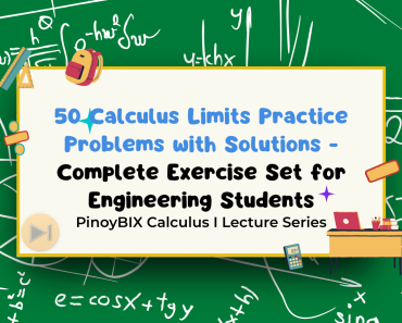
🎯Ready to Master Calculus Limits Through Practice?

Theory becomes expertise through application. Test your understanding with our comprehensive collection of 50 Calculus Limits Practice Problems with Solutions – featuring step-by-step solutions and complete explanations for engineering students.

From basic limit concepts to complex evaluation techniques, these exercises will solidify your calculus foundations and prepare you for advanced limit techniques ahead.

Join 1,000+ engineering students who’ve already mastered limits with PinoyBIX practice sets!

“These practice problems helped me ace my Calculus exam! The step-by-step solutions made everything click.” – Maria S., ECE Student

⭐⭐⭐⭐⭐ 4.9/5 stars from 500+ engineering students

Building Toward Advanced Techniques

While fundamental limit techniques provide essential computational tools, they reach their limitations when confronted with challenging mathematical scenarios. Consider these expressions that require more sophisticated approaches:

• lim[x→0] sin(x)/x (trigonometric indeterminate form requiring specialized techniques)
• lim[x→∞] (1 + 1/x)^x (exponential indeterminate form needing advanced methods)
• lim[x→0] [e^x – 1]/x (exponential indeterminate form requiring sophisticated evaluation)
• lim[x→0] x·sin(1/x) (oscillatory behavior needing squeeze theorem applications)

These expressions involve indeterminate forms and complex behaviors that cannot be resolved using basic limit techniques alone. Such precise limit evaluations require the complete toolkit of advanced methods to handle the mathematical complexity that arises in sophisticated engineering applications.

🚀 Looking Ahead: Lecture 2 Preview

Our next lecture, “Advanced Limit Techniques,” will extend your foundational limit mastery to handle the challenging scenarios that basic methods cannot resolve. You’ll learn:

L’Hôpital’s Rule Applications:

• Understanding indeterminate forms (0/0, ∞/∞, 0·∞, ∞-∞, 0^0, 1^∞, ∞^0)
• Applying L’Hôpital’s Rule systematically to resolve complex limit problems
• Recognizing when repeated applications are necessary for multi-level indeterminate forms
• Working with exponential and logarithmic transformations for challenging cases

Squeeze Theorem Mastery:

• Understanding the theoretical foundation and geometric interpretation of the squeeze theorem
• Applying squeeze theorem techniques to oscillatory and bounded functions
• Constructing appropriate bounding functions for complex limit scenarios
• Analyzing trigonometric limits that exhibit oscillatory behavior

Specialized Techniques:

• Trigonometric limit evaluation using fundamental trigonometric limits
• Infinite limit analysis and asymptotic behavior understanding
• Strategic algebraic manipulation for complex expressions
• Combining multiple advanced techniques for sophisticated limit problems

Engineering Applications:

• Signal processing applications involving sinc functions and Fourier analysis
• Control system stability analysis requiring complex limit evaluations
• Heat transfer and fluid dynamics problems with exponential decay behavior
• Economic modeling with growth and decay rate analysis

Preparation for Success

To maximize your learning in Lecture 2, ensure you can:

• Apply basic algebraic manipulation techniques confidently and systematically
• Recognize different types of indeterminate forms and unusual function behaviors
• Use factoring, rationalizing, and substitution methods from this lecture effectively
• Understand the geometric interpretation of limits and their connection to function behavior

The foundational mastery you’ve developed with basic limit techniques will make advanced limit evaluation work much more manageable and meaningful. The advanced techniques build directly on the systematic approach and algebraic skills developed in this lecture.

Final Thoughts

Remember that limit evaluation remains the fundamental computational foundation underlying all of calculus across every engineering discipline. Whether analyzing system response in control engineering, signal behavior in electrical systems, reaction rates in chemical processes, or optimization problems in industrial applications, these foundational limit techniques provide the mathematical rigor necessary for professional engineering practice.

The basic limit techniques you’ve mastered handle the computational foundation that makes advanced mathematical analysis possible. Combined with the sophisticated limit evaluation methods in our next lecture, you’ll possess the complete toolkit for understanding how complex mathematical behaviors are precisely analyzed and calculated.

Continue practicing these fundamental limit techniques systematically, understand the reasoning behind each method, and prepare to see how this computational foundation enables the mastery of advanced limit evaluation techniques that handle the most challenging mathematical scenarios in engineering analysis.

📌 SAVE this lecture for your next calculus study session!

💬 COMMENT below:

• Which fundamental concept from today’s introduction resonated with you the most?
• What real-world application of limits surprised you?
• Which basic technique do you want to see more examples of?

🔔 FOLLOW for more: Foundational calculus tutorials designed specifically for engineering students

📚 SHARE with: Your study group, classmates, or anyone just starting their calculus journey

🎓 Study Tip of the Day:

“Master the fundamentals first! Before jumping into complex problems, ensure you can quickly identify when to use direct substitution vs. algebraic manipulation. This decision-making skill is the foundation for all advanced limit work!”

Remember: Every calculus expert started exactly where you are now. Every engineering professional once struggled with their first limits. Build your foundation strong, practice consistently, and those challenging concepts will become intuitive!

See you guys in Lecture 2: Advanced Limit Techniques! 📈